
The field guide · Earth
Schumann resonance at Nagycenk
Nagycenk’s observatory in Hungary measures Schumann resonance with electric and magnetic field sensors. Its public chart shows three field components and estimates of the first three resonance modes.
 Open figure at full size ↗
Where is Nagycenk observatory?
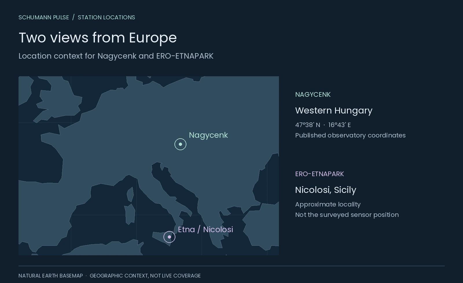
The station lies near Sopron in western Hungary, close to Lake Fertő. Its published coordinates are 47°38′ N, 16°43′ E; the observatory code is NCK. The current website identifies it as the HUN-REN EPSS Széchenyi István Geophysical Observatory. Official observatory information [1].
Our station explorer places it alongside Etna and Tomsk. Nagycenk’s own public Schumann resonance display (opens in a new tab) is the place to inspect its latest published chart. Read the date on the image before interpreting it as current.
 Open figure at full size ↗
From geophysics to continuous resonance records
The observatory began supplying geophysical data in 1957, during the International Geophysical Year. Its early work included earth-current observations; resonance measurements arrived decades later. Observatory history [5].
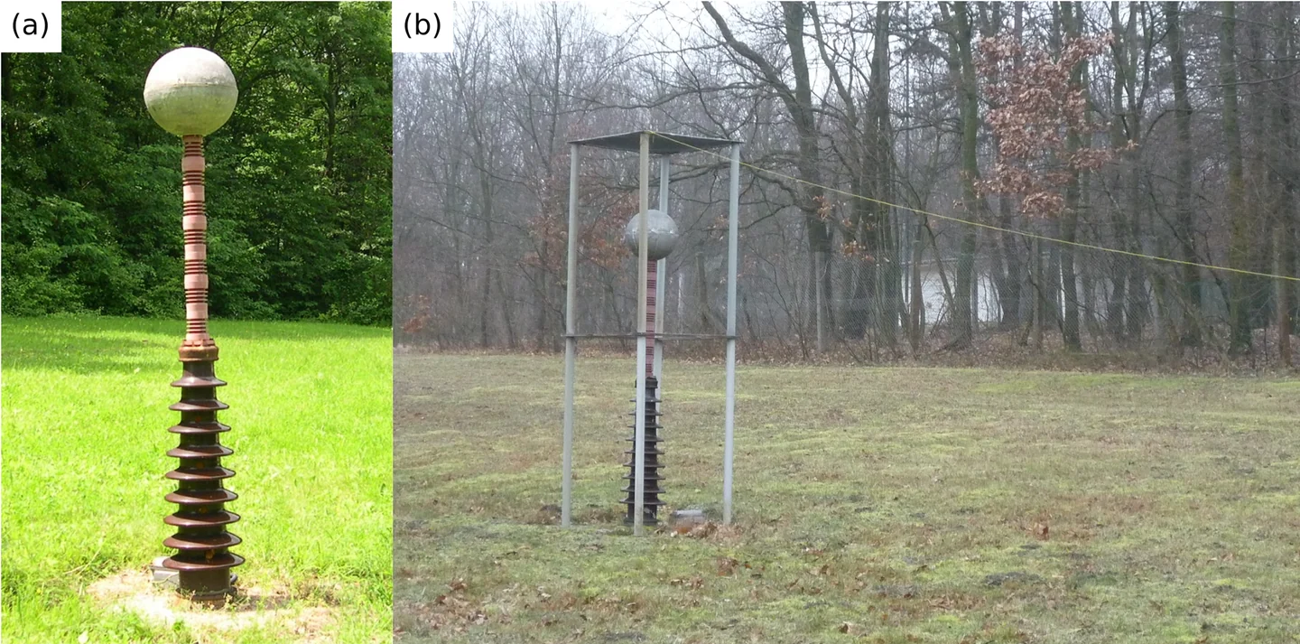
Antal Ádám and Pál Bencze attempted resonance detection in the 1960s using an L-shaped antenna and a tape recorder. Gabriella Sátori later advanced continuous monitoring. A new ball antenna enabled regular spectral-parameter records from May 1993; magnetic coils followed in 1996. These dates come from the research team’s 2020 historical review, section 3.1 [6].
The photograph above shows that ball antenna and a calibration arrangement dated 20 December 2013. The metal sphere senses the electric field; it is not a broadcasting antenna or a device that generates Earth’s resonance. The authors describe a roughly 200 kg assembly designed to reduce mechanical vibration. Calibration applies a known test field so the instrument’s response can be assessed. Bór and colleagues, instrument description and Figure 9 [6].
What do the three channels mean?
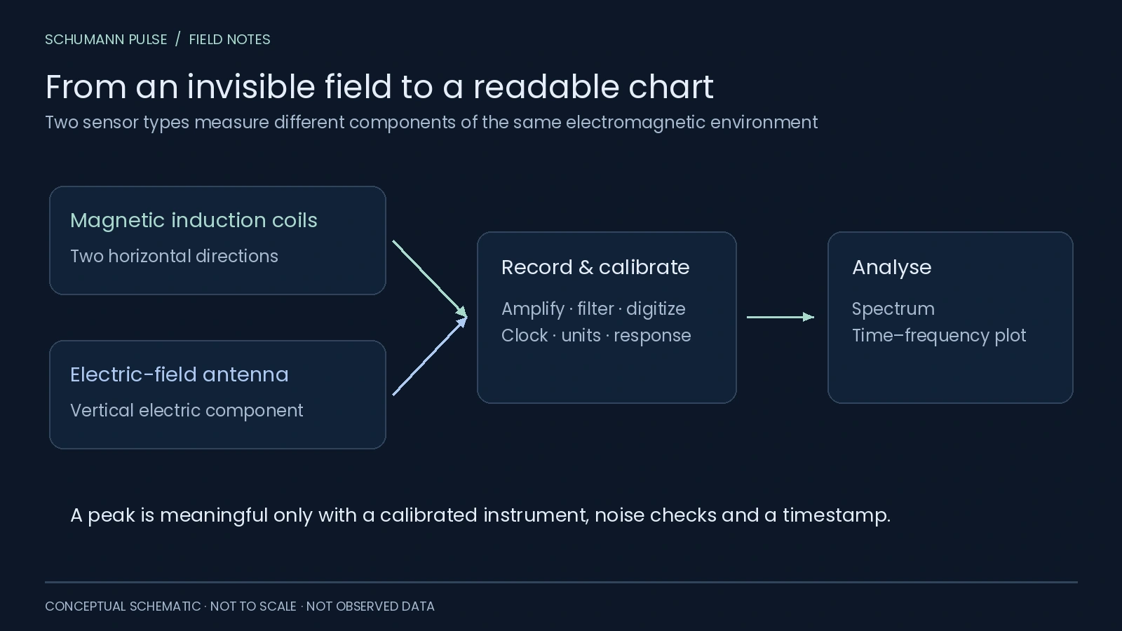
The display documentation distinguishes three field components:
Swipe or use the arrow keys to see all columns.
| Label | Measurement |
|---|---|
| H_NS | Horizontal magnetic component along north–south |
| H_EW | Horizontal magnetic component along east–west |
| E_Z | Vertical electric component |
Its two additional panels estimate amplitude and frequency for the first three modes from E_Z. Frequency identifies a peak’s position in hertz; amplitude describes its size on the stated scale. They answer different questions. Automatic display technical report [7].
 Open figure at full size ↗
How should I read the public chart?
Start with the timestamp, then identify the component, frequency axis and colour scale. The technical report describes different scales for the two magnetic channels. A brighter colour in one panel therefore does not, by itself, establish a larger physical signal than in the other.
The authors also caution that wind, precipitation and local electrical interference can bias automatic estimates. Quick-look values need quality checks before scientific interpretation. Processing and limitations, pages 36–38 [8].
For a practical walkthrough of bands, broad vertical features and gaps, see how to read a Schumann resonance chart. When comparing stations, keep a short checklist: same time interval, same field component, compatible units and documented processing. Our website does not combine Nagycenk’s chart with Tomsk’s numerical A1 series.
Can I download numerical data?
The published workflow describes internal CSV files feeding the chart. It does not provide an open CSV endpoint. Schumann Pulse currently links to the operator’s display; a Nagycenk numerical feed and daily comparison are not connected. Display workflow [8].
You can still use the Nagycenk station page to reach the source, or explore Etna’s magnetic-field observations to see another instrument’s view.
Sources
References in the text lead here. Original publications open in a new tab; this guide stays open.
Source review: 21 October 2026. Historical dates describe the cited publications; they are not a guarantee of uninterrupted recording today.
- [1] Nagycenk official site: identity, coordinates and public display (opens in a new tab) Back to text ↑.
- [2] Bór et al. (2020): station history, instruments and Figure 9 (opens in a new tab), CC BY 4.0.
- [3] Szabóné André et al. (2021): automatic ELF display and quality limitations (opens in a new tab).
-
[4] Natural Earth: public-domain map geometry (opens in a new tab).
-
[5] Observatory history (opens in a new tab) Back to text ↑.
- [6] Bór et al.: full historical review (opens in a new tab) First mention ↑.
- [7] Automatic display report (opens in a new tab) Back to text ↑ and [8] full technical text (opens in a new tab) First mention ↑.
Keep exploring
Make room for your own observations.
Schumann Pulse brings environmental readings and your personal journal into one place. The app is coming soon for iPhone.
Explore the app