
The field guide · Earth
Why do Schumann resonance stations show different readings?
Schumann resonances belong to the global Earth–ionosphere system, but a station records them through a local instrument. Lightning geometry, the measured field component, calibration and chart processing can make station records differ. There is no single worldwide amplitude number.
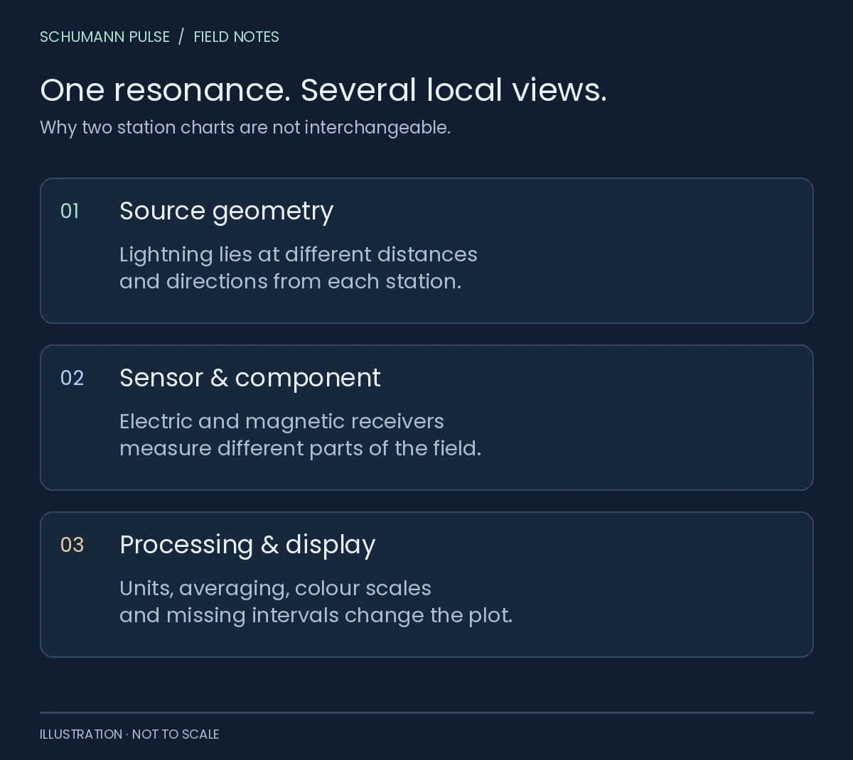
Schumann Pulse · field notes
One resonance. Several local views.
Why two station charts are not interchangeable.
Source geometry
Lightning lies at different distances and directions from each station.
Sensor & component
Electric and magnetic receivers measure different parts of the field.
Processing & display
Units, averaging, colour scales and missing intervals change the plot.
Original comparison framework. No station readings are plotted; no cross-station calibration is implied.
A global phenomenon is not an identical local signal
Imagine asking three cameras to describe the same landscape from different positions. The analogy is limited, but it helps distinguish a shared phenomenon from a shared recording. For Schumann resonance, the relevant differences include the location of lightning relative to each receiver and the field component it measures.
Sátori and colleagues studied how lightning-source geometry affects peak frequencies in Nagycenk’s vertical electric-field record. Their 2024 paper considers several time scales and a moving South American thunderstorm system. It shows why a measured spectral peak need not behave as a universal fixed clock. It does not establish one conversion rule for every electric and magnetic station. Sátori et al., 2024 [1].
Electric and magnetic measurements are different
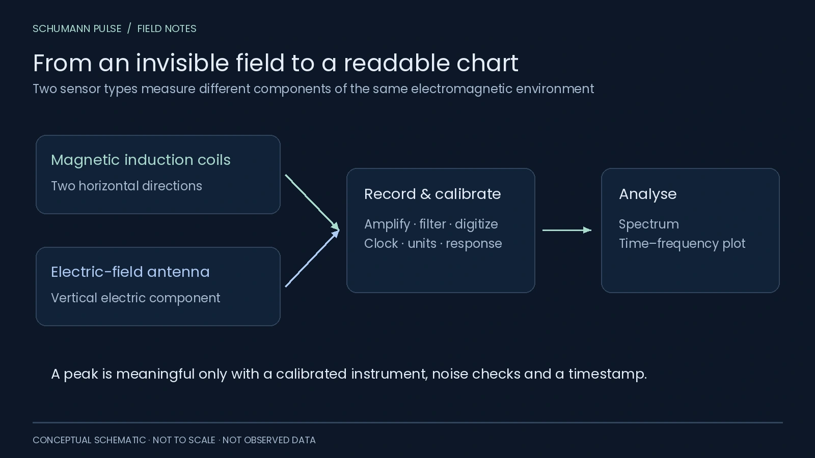
Nagycenk’s documentation names E_Z, the vertical electric component, and two horizontal magnetic components, H_NS and H_EW. Its displayed mode amplitudes and frequencies are extracted from E_Z. Etna’s documented EC200 is an induction-coil magnetic receiver. Nagycenk display report [2] and Etna instrumentation [4].
An electric-field amplitude cannot simply be placed on a magnetic-field axis. Even two magnetic channels may have different orientations, response functions or noise. A fair comparison starts with the measurement definition, not the colours.
 Open figure at full size ↗
What the three station views actually offer
Swipe or use the arrow keys to see all columns.
| Station | Documented public context | How we use it |
|---|---|---|
| Tomsk | Source amplitude/frequency series and station metadata | A separately labelled current numerical record; its A1 scale is not a universal Earth score |
| Nagycenk | Electric and magnetic spectrograms; extracted E_Z mode parameters | Station context and a link to its public display; no numerical feed connected here |
| Etna | EC200 magnetic spectrograms | Attributed current source image and station context; no numerical feed connected here |
These describe our integration status at the editorial review date, 22 October 2026, not a claim that all stations are online continuously. The station explorer labels the selected source and available view. Its map markers are locations, not a spatial heatmap of resonance intensity.
Before comparing two charts, check five things
- Time. Convert both axes to the same time zone and compare overlapping intervals. Retrieval time is not observation time.
- Component. Identify electric or magnetic field and sensor orientation.
- Units. Separate amplitude, power, spectral density and frequency. They are not interchangeable quantities.
- Processing. Check averaging, filtering and how a peak was estimated. Nagycenk’s automatic display report explains its own processing and interference limitations.
- Display. Read each colour scale and identify gaps or clipping before judging intensity.
A hypothetical bright white patch on one plot and a green band on another cannot settle which measured a larger signal if the scales differ. Likewise, an empty interval does not establish zero resonance. The whiteout and blackout guide shows the same invented values with two colour scales and separates missing data from low readings.
Does disagreement mean a station is wrong?
Not necessarily. Instrument noise, local conditions and real differences in response all need consideration. Nagycenk’s historical review describes the development and calibration of its instruments, illustrating how much work sits behind a seemingly simple chart. Bór et al., 2020 [3].
A scientific cross-station analysis needs calibrated, quality-controlled data and a stated method. Our source-specific views help you inspect the available evidence; they do not merge incompatible records into a global “energy” score or a personal health assessment.
Sources
References in the text lead here. Original publications open in a new tab; this guide stays open.
- [1] Sátori et al. (2024): lightning geometry and Nagycenk E_Z peak frequencies (opens in a new tab) Back to text ↑.
- [2] Szabóné André et al. (2021): Nagycenk display, components and processing (opens in a new tab) Back to text ↑.
- [3] Bór et al. (2020): station history and instruments (opens in a new tab) Back to text ↑.
- [4] ERO-ETNAPARK: EC200 receiver and display descriptions (opens in a new tab) Back to text ↑.
- [5] Tomsk source operator (opens in a new tab).
Your next observation
Put a reading beside your own experience.
Record how you feel, with optional energy, mood and focus ratings. Revisit your entries alongside dated station readings and explore comparisons when enough suitable records are available.
iPhone app coming soon · history and personal comparisons live in the app.